File under Dept. of random observations: many have stumbled upon the inability for artificial intelligence to do well in low dimensional areas where much is unknown. I still feel this is the most interesting frontier of human endeavors. It’s always been there, it just got a little blurry for a moment.

-
Biological complexity File under Dept. of random observations: many have stumbled upon the inability for artificial intelligence to do well in low dimensional areas where much is unknown. I still feel this is the... Read more
-
Fundamentals of causal inference: part 1 Preliminary definitions and assumptions, causal inference assumptions, incident user and active comparator designs. Read more
Introduction
I became interested in causal inference after noticing differences between causality in the field of causal inference, and causality in pathogen transmission mechanistic models. I find the definitions and formalities in causal inference, and statistics more generally, satisfying.
One of the most fun things about the history of statistics is how rich it is with interesting anecdotes and case studies. I enjoyed listening to Prof. Susan Ellenberg’s recounting of its history.1 It’s interesting to think about modern clinical trials only gaining traction in the mid-twentieth century, and the human complications that arise when putting these designs into practice. For instance, is it ethical to have placebo groups if the treatment has the potential to save the life of the participant? At what points should trials stop if we think the treatment is having a positive effect? When vaccines are used widely, and therefore a rare bad health event coincidentally occurs shortly after a baby is vaccinated, what is the best way to address, with scientific evidence, the concerns of a parent? What was also interesting was hearing about the difference between an active control vs. a placebo control, and how even studies where the treatment has a known effect may fail. By it’s very nature of applying abstract theory to real-world situations, and encountering all sorts of complications, the statistical literature is full of interesting human stories.
The following is adapted from module one of Prof. Jason Roy’s fantastic online Coursera course on causal inference https://www.coursera.org/learn/crash-course-in-causality.2 I wanted to review the basics of causal inference for myself. I recall a professor in undergrad saying that one should never underestimate the fundamentals. This is part one of five.
Preliminary definitions and assumptions
Suppose we are interested in the causal effect of some treatment \(Z\) on some outcome \(Y\). For example, \(z = 1\) indicates an individual taking a vaccine against influenza and \(Z = 0\) otherwise; \(Y\) is the time until the individual is infected. We can notate \(Y(Z = 1)\) and \(Y(Z = 0)\) as potential outcomes given treatment.
A counterfactual outcome is the outcome that would have been observed with the treatment had been different. For example, if the treatment of an individual was \(Z = 0\), then the counterfactual outcome would be \(Y(Z = 1)\) and vice-versa. Before treatment assignment, any outcome is a potential outcome, but after the study there is an observed outcome and a counterfactual outcome. It is normally assumed that counterfactual outcomes are the same as potential outcomes.
It is important that there is clearly one treatment, and that there are no hidden treatments in the mix. For example, we may be interested in the causal effect of BMI on some health outcome. The problem is that there are many potential ways to achieve a particular BMI value, which can lead to different outcomes. Similarly, some variables are simply immutable, such as race. Because race is not manipulable, we cannot identify a causal effect for it. These causal effects certainly exist, but are not easily identified within the causal inference framework.
A causal effect is identified if there is a difference in \(Y(Z = 1)\) and \(Y(Z = 0)\). However, for any individual we can only ever observe one of these potential outcomes. This is what is known as the fundamental problem of causal inference. We get around the problem by considering population-level causal effects rather than individual-level causal effects, where \(Y(Z = 1)\) would be the averaged outcome of all individuals if all individuals were assigned treatment \(Z = 1\).
We should note that \(E[Y(Z = 1) - Y(Z = 0)] \neq E[Y \mid Z = 1] - E[Y \mid Z = 0]\). This is because in reality there may be differences in the population that had \(z = 1\) vs. \(z = 0\); for example, individuals at a higher risk for flu may be more likely to get a flu shot, so this may differ from what would happen if all individuals were either assigned to \(Z = 1\) or \(Z = 0\). Generally, if we are comparing two different populations, then we are not identifying a causal effect, whereas we would be identifying the causal effect if we compare the same population where the only difference is treatment.
Causal inference assumptions
These are:
- Stable Unit Treatment Value Assumption (SUTVA), which allows us to write the potential outcomes for individual \(i\) in terms solely of the treatment individual \(i\) receives
- No interference: units do not interfere with each other, where the treatment of one individual does not affect the outcome of another
- One version of treatment
- Consistency
- The potential outcome \(Y(Z)\) is equal to the observed outcome if the actual treatment received is \(Z = z\). In other words \(Y = Y(Z)\) if \(Z = z\) for all \(z\).
- Ignorability (sometimes referred to as the no unmeasured confounders assumption)
- Given pre-treatment covariates \(X\), who is treated (treatment assignment) is independent from the potential outcomes (formally: \(Y(0), Y(1) \perp\!\!\!\perp Z \mid X\)). For instance, maybe sicker individuals are assigned treatment more often than less sick individuals, and they are also more likely to have a bad outcome. In this case, who is treated \(Z\) is not independent of the potential outcomes (note that if treatment assignment is randomized no matter the sickness of the individual we wouldn’t have a problem). We are looking for: within each stratum of \(X\) (in this case age) treatment \(Z\) is randomly assigned, so that potential outcomes within each stratum are independent of treatment assignment.
- Positivity
- \(P(Z = z \mid X = x) > 0 \;\; \forall z \text{ and } x\). In other words, the probability of treatment assignment is positive no matter your covariate values of \(X\).
We can get from the observed outcome to the potential outcome through the following proof: \(E[Y \mid Z = z, X = x]\) involves only observed data. \(E[Y \mid Z = z, X = x] = E[Y(z) \mid Z = z, X = x]\) by consistency. \(= E[Y(z) \mid X = x]\) by ignorability.
If we want a marginal causal effect we can average over the distribution of \(X\). Suppose \(X\) is a single categorical variable, then \(E[Y(z)] = \sum_x E[Y \mid Z = z, X = x] \Pr(X = x)\). This process is known as standardization, which involves stratifying then averaging. In other words we obtain a treatment effect within each stratum then pool across stratum, weighting by the probability (or size) of each stratum. We can follow this procedure with the real data. As long as there is randomization of treatment assignment within each stratum, we can identify a causal effect.
Standardization can be difficult if there are many \(X\) variables needed to achieve ignorability, and if there are many empty cells of combinations of \(X\) variables. Because of this difficulty, much work has been done on remedies such as matching, inverse probability of treatment weighting, propensity scores, and instrumental variables.
Incident user and active comparator designs
Suppose we were interested in the effect of yoga on blood pressure. If we take a cross-section of five people, we might find that two of them are currently practicing yoga and three are not. However, there may be variable individual histories of whether they ever did yoga in the past, which creates complications if we want to compare a group that does currently practice yoga vs. doesn’t.
One way to get around this would be an incident user study design, where we restrict the treated population to those newly initiating treatment. In this way, we would ask the slightly different causal question of: for the population of individuals who have not practiced yoga in the past, what is the causal effect of practicing yoga.
One last challenge is that although start of follow-up time of treated individuals is clear, i.e., when they initiate yoga, it is less clear what the start of follow-up time is for the control. In this case, we might want to have an active comparator control, such as Zumba, which would also have a clear start of follow-up time. There is normally less confounding when using an active comparator, but the causal question becomes more narrow. Finally, active comparators may not be possible, or even what we are interested, so they don’t always have to be used.
References
- S. Ellenberg. People & perspectives: Susan Ellenberg. https://www.youtube.com/watch?v=aMkO5vezUcs.
- J. Roy. A crash course in causality: Inferring causal effects from observational data. https://www.coursera.org/learn/crash-course-in-causality.
- Stable Unit Treatment Value Assumption (SUTVA), which allows us to write the potential outcomes for individual \(i\) in terms solely of the treatment individual \(i\) receives
-
Fundamentals of causal inference: part 2 Confounding, DAGs, controlling for confounders. Read more
Introduction
The following is adapted from module two of Prof. Jason Roy’s online Coursera course on causal inference https://www.coursera.org/learn/crash-course-in-causality.1 I wanted to review the basics of causal inference for myself. This is part two of five.
Confounding
Confounding occurs when some factor affects both the treatment and outcome. For example, if in a trial older people are more likely to receive a particular treatment for cardiovascular disease, as well as have higher risk for cardiovascular disease, then age would be a confounder. In contrast, if age solely increases the risk for cardiovascular disease (the outcome) and not the treatment assignment, this would not be a confounder. If just the treatment is based on some factor, but not the outcome is not dependent on this factor, this would also not be a confounder. To control for confounding, we are interested in a set of variables \(X\) that will allow us to achieve ignorability, or independence between the potential outcomes and the treatment assignment.
Preliminary: DAGs
One way for us to keep track of controlling for confounding is to use causal graphs diagrams. We use directed-acyclic graphs (DAG). If we have:
\[D \rightarrow A \rightarrow B \quad C\]Then we know certain relationships between the variables:
- \(P(C \mid D, A, B) = P(C)\), i.e., \(C\) is independent of all variables
- \(P(B \mid D, A, C) = P(B \mid A)\), i.e., \(B \perp\!\!\!\perp D, C \mid A\)
- \(P(B \mid D) \neq P(B)\), i.e., \(B\) and \(D\) are marginally dependent
- \(P(D \mid B, A, C) = P(D \mid A)\), for similar reasons as for point two
Here is another example:
\[A \leftarrow D \rightarrow B \rightarrow C\]Where we know the following relationships:
- \(P(A \mid D, B, C) = P(A \mid D)\), i.e., \(A \perp\!\!\!\perp B, C \mid D\)
- \(P(D \mid A, B, C) = P(D \mid A, B)\), i.e., \(D \perp\!\!\!\perp C \mid B\)
Given a DAG we can decompose the joint distribution. We do this by starting with the roots of the DAG and writing down any dependencies of each child (note: if a child has two parents then we need to condition on both parents). For example in the first example the joint distribution would be \(P(A, B, C, D) = P(C)P(D)P(A \mid D)P(B \mid A)\). The joint distribution of the second example would be \(P(A, B, C, D) = P(D)P(A \mid D)P(B \mid D)P(C \mid B)\). We say that a DAG and a joint distribution are compatible. For a given DAG, we can write down its joint distribution function, but a given joint distribution may not necessarily be unique to one DAG.
Some examples of other terms to know:
- Fork: \(A \leftarrow D \rightarrow B\)
- Note that \(A\) and \(B\) are not independent because information flows from \(D\) to both
- Chain: \(A \rightarrow D \rightarrow B\)
- Again, here \(A\) and \(B\) are not independent
- Inverted fork: \(A \rightarrow D \leftarrow B\)
- Here \(D\) is a collider. \(A\) and \(B\) are independent because there is no information flow between them. If you were to condition on \(D\), you would create an association between \(A\) and \(B\). Imagine \(A\) and \(B\) are light switches that are determined by coin flips and \(D\) is whether a lightbulb is on, and it can only be on if both \(A\) and \(B\) are on. If we know the condition of \(A\) this doesn’t tell us anything about \(B\) and vice-versa. However, if we know the lightbulb is off, then we know that \(A\) must be on if \(B\) is off and vice-versa.
- Blocking: \(D\) is blocking the path \(A \rightarrow D \rightarrow B\).
- Imagine \(A\) is temperature, \(D\) is icy sidewalks and \(B\) is if someone falls. Here \(D\) and \(B\) are marginally associated. But if we condition on \(A\), then \(D\) and \(B\) are not associated according to this path. This can also occur on a fork like \(A \leftarrow D \rightarrow B\).
A path is d-separated by a set of nodes \(C\) if for all chains and forks it contains the middle part of each, and for inverted forks it does not contain the middle part nor any descendants of the middle part. Two nodes \(A\) and \(B\) are said to be d-separted by a set of nodes \(C\) if every path from \(A\) to \(B\) is blocked. We attempt to create conditional independence by blocking (controlling) for \(C\) i.e., \(A \perp\!\!\!\perp B \mid C\).
Controlling for confounders
Now that we’ve learned all about DAGs we can think about how to control for confounders. We just need a bit more terminology to do so:
- Frontdoor path: a path that emanates out of treatment to outcome such as \(Z \rightarrow Y\) or \(Z \rightarrow W \rightarrow Y\). These paths capture effects we want to measure such as the effect of treatment on the outcome. Note that if we are interested in the effect of \(Z\) on \(Y\) through \(W\) then this would be a causal mediation analysis.
- Backdoor path: a path that travels from \(Z\) to \(Y\) through an arrow that goes into \(Z\). For example if \(Z \rightarrow Y\) and \(Z \leftarrow X \rightarrow Y\) then \(X\) would be a backdoor path. Backdoor paths confound the relationship between \(A\) and \(Y\).
We will need to block the backdoor paths in order to control confounders so that ignorability holds. We have two criterion that let us know if we have successfully controlled for confounders.
Backdoor path criterion
A set of variables \(X\) is sufficient to control for confounding if (1) it blocks all backdoor paths from treatment to outcome and (2) it does not include any descendants of treatment. Note that \(X\) is not necessarily unique.
Some examples of how to satisfy the backdoor path criterion:
- \(Z \rightarrow Y\) and \(Z \leftarrow V \rightarrow W \rightarrow Y\). There is one backdoor path to block, which we can block with \(V\) or \(W\) or both.
- \(Z \rightarrow Y\) and \(Z \leftarrow V \rightarrow M \leftarrow W \rightarrow Y\). Here there is a collider \(M\) so there is actually no confounding. As long as there is no information flow along a backdoor path, then \(Z\) is not associated with \(Y\) through the backdoor path and there is no confounding. If \(M\) was controlled you could unintentionally open up a path that would need to be controlled.
Strategy for controlling for backdoor paths: for each backdoor path, check if they have colliders or not. If they do then nothing to worry about. If they don’t then control for something on the path that will block the path. Of the conditions to block each path, find the minimal set where all backdoor paths are blocked.
In practice, people come up with very complicated graphs which need to be controlled. Case in point:
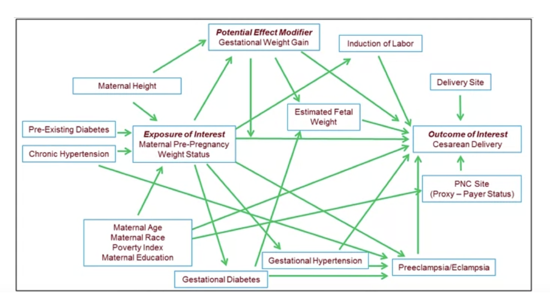 Figure S1: DAG between maternal pre-pregnancy weight and risk of C-section. Reproduced from Figure 1 of Vahratian et al. (2005).
Disjunctive cause criterion
Suppose we don’t know the true DAG. We can choose to use the disjunctive cause criterion which is simply to control for all observed causes of the exposure, outcome or both. This is due to the property that if there is a set of observed variables that satisfy the backdoor path criterion then the variables selected by the disjunctive cause criterion will be sufficient to control for confounding.
Here is a simple example: suppose we know pre-treatment variables \(M, V\), and \(W\) and unobserved pre-treatment variables \(U_1\) and \(U_2\). Suppose we know \(W\) and \(V\) are causes of \(Z\), \(Y\) or both and \(M\) is not. Suppose we don’t know the DAG. We can use the disjunctive cause criterion and can control for \(V, W\) and this would be sufficient. Thus, we simply need to note which variables cause the treatment, outcome, or both, and which do not. If we simply controlled for all pre-treatment variables, due to unobserved pre-treatment variables we can unintentionally not satisfy the backdoor path criterion.
We should note that there could be a case where the backdoor path criterion cannot be satisfied simply through controlling the observed pre-treatment variables due to the unobserved pre-treatment variables not being controlled, and in this case the disjunctive cause criterion would also fail. Similarly, we also need to know all causes of \(A\) and \(Y\) for the disjunctive cause criterion to work. We also note that the disjunctive cause criterion set is not always smaller than the backdoor path criterion set.
References
- J. Roy. A crash course in causality: Inferring causal effects from observational data. https://www.coursera.org/learn/crash-course-in-causality.
-
Fundamentals of causal inference: part 3 Observational studies, matching, analyzing matched data, propensity scores. Read more
Introduction
The following is adapted from module three of Prof. Jason Roy’s online Coursera course on causal inference https://www.coursera.org/learn/crash-course-in-causality.1 I wanted to review the basics of causal inference for myself. This is part three of five.
Observational studies
Observational studies differ from randomized trials. They are subject to confounders, since treatment has not been randomized. Imagine \(Z \rightarrow Y\) and \(Z \leftarrow X \rightarrow Y\). In this scenario, what randomization effectively does is eliminate \(Z \leftarrow X\) so that there are no backdoor paths from \(Z\) to \(Y\) so that ignorability is satisfied. More specifically, the distribution of \(X\) is now randomly distributed to both treatment groups, i.e., the marginal distribution of \(X\) is the same as the distribution of \(X\) given \(Z = 1\) or \(Z = 0\). This is known as covariate balance, and is dealt in the design phase.
So why not randomize everything? Because randomized trials are very expensive and lengthy, or could be unethical (e.g., randomizing people to smoke), or people might not want to have the chance to receive a placebo thus shrinking the study population. Planned, prospective observational studies could be used instead, although of course there are drawbacks such as low data quality, and they can still at times be expensive.
Matching
Description
Matching is a way that observational studies try to address confounding. Imagine \(X\) is age, and older people are more likely to have \(Z = 1\) and younger people are more likely to have \(Z = 0\). In matching, we try to find, for each treated person \(Z = 1\) of a certain age, we try to find an untreated person \(Z = 0\) with the same age to perform a comparison. In a randomized trial for any age we would expect to find about the same number whether \(Z = 1\) or \(Z = 0\). Matching tries to achieve this.
Matching is nice because we can do it before looking at outcomes, as it is still done in the design phase. It can also reveal whether, for example, some ages had no chance of receiving treatment, and we would try to exclude them from the study since we don’t want to make inference on people who had no chance of either receiving treatment or not receiving treatment as this would violate the positivity assumption.
What occurs more specifically in matching is that we match a person with \(Z = 1\) and a given \(X\) to a person with \(Z = 0\) with the same \(X\). Individuals in the smaller group will try to find matches in the bigger group; usually the treatment is the smaller group and control is the bigger group. Then we get rid of all the others that didn’t have a match.
We will not be able to exactly match on the full set of covariates, for example maybe we couldn’t find an exact match of age 55 in the control, but we could find an age 56, which may be close enough. But even in randomized trials we may not have exact matches, we have stochastic balance. Matching will also try to achieve stochastic balance.
It’s subtle, but matching will only provide us with the causal effect of treatment on the treated, since we are finding matches in the control group that match individuals in the treatment group. That is, if we took individuals from the treated population, not the whole population, we ask the causal question of what would happen to them if \(Z = 0\) or \(Z = 1\). So we’re not trying to match the distribution of \(X\) to the marginal distribution of \(X\) across treatment groups.
Sometimes it is difficult to find great matches. For example, if a treated male of age 40 is matches to a control female of age 45 and a treated female of age 45 is matched to a control male of age 40, this would not have stochastic balance. However, this does have fine balance since the distribution of \(X\) is the same among treated and control.
There’s also a question of how many matches to make. For example, although so far we’ve done one to one matching, we can also do five to one matching where for every treated individual we can match them to five control individuals.
How do we create good matches?
We can create good matches by creating distance matrices between individuals based on their \(X\) covariates. There is the Mahalanobis distance (M distance) and robust Mahalanobis distance (robust M distance). Denote \(X_j\) as a vector of covariates for subject \(j\). The Mahalanobis distance between subject \(i\) and \(j\) is:
\[D(X_i, X_j) = \sqrt{(X_i - X_j)^T S^{-1} (X_i - X_j)}\]Where \(S\) is the symmetric covariance matrix of \(X\), which is done to scale the variables. So in the first matrix multiplication its looking at the difference in the first variable of \(X_j\) and then scaling by the variance of the first variable with itself plus the difference in the second variable with the second variable of \(X_j\) and then scaling by the covariance between the first variable and second variable, etc. for all other differences of the other variables and covariance with the first variable. Essentially we square the differences of each variable, scale by the covariance, and take the square root.
The robust Mahalanobis distance tries to account for the fact that outliers can create large distances, so we might be better off trying to match the ranks. One subtlety is that the diagonal of the covariance matrix will be a constant.
Greedy (nearest-neighbor) matching First, imagine the pool of control subjects is much larger than for treated subjects, which is often the case. The algorithm is:
- Randomly order list of treated subjects and control subjects
- Start with first treated subject. Match to control with the smallest distance (this is greedy)
- Remove the matched control from the list of available matches
- Move on to next treated subject and repeat for all treated subjects
This is intuitive and computationally fast, but it depends on the initial order of the list, and may not be globally optimal.
This is the algorithm for pair-matching, but for many to one matching the algorithm would slightly change to first find matches for all treated subjects, then go back and find second matches for all treated subjects. Many to one matching may be preferred since it uses more control subjects, but it may also lead to worse matches. There is essentially a bias-variance tradeoff where there may be closer matches in pair matching but larger variance, and vice-versa in many to one matching.
A caliper is a maximum acceptable distance to avoid very bad matches. This gets back to the positivity assumption, since probability of each treatment should be non-zero.
Optimal matching Finding the global optimal match is computationally expensive, but R packages have been developed to do this. But it also depends on the size of the problem. For example even if there are a million possible pairings (e.g. 1000 possible treated and 1000 possible control) this should still be runnable. We can constrain the number of pairings by blocking globally optimal matches within certain subsets, subpopulations, of the data (also known as sparse matching).
To assess the balance we can look for example at the means of the covariates and see whether they are similar between the two groups before and after matching. We can also take a look at the standardized difference between the two groups:
\[smd = \left| \frac{\overline{X}_{treatment} - \overline{X}_{control}}{\sqrt{\frac{s^2_{treatment} + s^2_{control}}{2}}} \right|\]Where values \(< 0.1\) indicate adequate balance, values between 0.1 and 0.2 are O.K. and values greater than 0.2 indicate imbalance.
Analyzing matched data
Imagine we’ve successfully matched the data. We can analyze the data with permutation tests. The main idea is to first create a test statistic from the observed data, such as a difference in sample means between the two groups. Then assume the null hypothesis of no treatment effect is true. Randomly permute the treatment and control labels for each pair and calculate the test statistic, and do this thousands of time to create a null distribution. Then check whether the observed test statistic is unusual compared to the null distribution. A McNemar test can also be used for paired data or a paired t-test for continuous data that tests against the null of no difference between the treatment conditions of each pair. There are also more complicated models that can be used such as a conditional logistic regression, stratified Cox model, and generalilzed estimating equations (GEE).
Sensitivity analyses should also be done for analysis. In observational studies especially, there may be hidden biases where the ignorability assumption is violated. For observational studies we can determine if there is hidden bias, how severe would it have to be for us to change conclusions? Let \(\pi_j\) and \(\pi_k\) be the probabilities that person \(j\) and \(k\) receive treatment. Suppose person \(j\) and \(k\) are perfectly matched so that the observed covariates \(X_j\) and \(X_k\) are the same. If \(\pi_j = \pi_k\) then there is no hidden bias. Consider:
\[\Gamma = \frac{\frac{\pi_j}{1 - \pi_j}}{\frac{\pi_k}{1 - \pi_k}}\]The numerator is the odds of treatment for person \(j\) and the denominator is the odds of treatment for person \(k\). \(\Gamma\) is an odds ratio. If \(\Gamma = 1\) then there is no overt bias and \(\Gamma > 1\) or \(\Gamma < 1\) implies hidden bias. So we can increase \(\Gamma\) until the conclusion changes due to, for example, a wider range of p-values at some level of \(\Gamma\) that cross the \(\alpha = 5\%\) significance level. For an example of how the computation for this is done for the Wilcoxon-signed rank test, which essentially gives a range for the null-distribution depending on \(\Gamma\) see Rosenbaum (2005).2 The point at which the conclusion changes due to a bias in the odds of treatment assignment gives us some sense of how sensitive our results are to hidden biases: for example if \(\Gamma = 1.1\) for the conclusion to change, then this is very sensitive to confounding, compared to if conclusions change when \(\Gamma = 5\), since the latter is saying that there must have been a confounder that assigned treatment 5 times more often to treatment than control to change the result.
Propensity scores
A propensity score is the probability of receiving treatment rather than control given covariates \(X\). That is, for subject \(i\):
\[\pi_i = P(Z = 1 \mid X_i)\]To make it more concrete, if older people were more likely to get treatment, then \(\pi_i > \pi_j\) if \(age_i > age_j\).
Two individuals, \(i\) and \(j\) where \(X_i \neq X_j\) may still have \(\pi_i = \pi_j\), so they are just as likely to be found in the treatment group. If we only look at a subpopulation of subjects with the same \(\pi_i\), there should be balance in the two treatment groups. In this case the propensity score is a balancing score. More formally:
\[P(X = x \mid \pi(X) = p, A = 1) = P(X = x \mid \pi(X) = p, A = 0)\]If we match on the propensity score, rather than the raw covariate \(X\) as before, we should achieve balance, since the individuals of the treatment and the control should have had equal probability of being included in either the treatment or control group. In other words the probability of treatment is random given \(X\) if we match on the propensity scores. Note though that the propensity scores will not be randomly allocated to both groups since higher propensity scores should be seen more often in treatment since they are have a higher probability of being in the treatment group. Furthermore in theory the above states that the distribution of \(X\) given \(\pi(X) = p\) should be the same for both groups if we match on the propensity scores. Conditioning on the propensity score is conditioning on an allocation probability.
In a randomized trial the propensity score is known, but in an observational study it is unknown, but we can estimate it. Treat the treatment as an outcome: \(P(Z = 1 \mid X)\). We can fit a logistic regression model of \(Z\) vs. \(X\). From the model we can get a predicted probability for each subject, which is the estimated propensity score. This is very efficient to match on since we just have to match on a single variable for balance rather than balancing all covariates.
Before we match we need to look for overlap, where in the distribution of the propensity score among the two groups, there is always positivity no matter the propensity score. We could also check to see that there ended up being a higher peak among treated individuals, since they were more likely to have a higher probability of receiving treatment. Sometimes there is poor overlap at the tails, but causal effects can be estimated where there is overlap and trimming off these tails, and satisfying the positivity assumption. In practice we can also transform the propensity score to the log-odds to “stretch” the distribution, so we would match on \(logit(\pi)\) rather than \(\pi\), as well as use a caliper that is 0.2 times the standard deviation of the logit of the propensity score, although this is somewhat arbitrary. A smaller caliper has less bias, but more variance.
Then like before a randomization test for analysis can be used after matching on the propensity scores.
References
- J. Roy. A crash course in causality: Inferring causal effects from observational data. https://www.coursera.org/learn/crash-course-in-causality.
- Paul R Rosenbaum. Sensitivity analysis in observational studies. Encyclopedia of statistics in behavioral science, 4:1809–1814, 2005.
-
Fundamentals of causal inference: part 4 Inverse probability of treatment weighting (IPTW), marginal structural models, IPTW estimation, weights, doubly robust estimators. Read more
Introduction
The following is adapted from module four of Prof. Jason Roy’s online Coursera course on causal inference https://www.coursera.org/learn/crash-course-in-causality.1 I wanted to review the basics of causal inference for myself. This is part four of five.
Inverse probability of treatment weighting (IPTW)
Imagine that the propensity scores for some covariate \(X\) is \(P(Z = 1 \mid X = 0) = 0.1\). Then it is likely that most of them will be assigned to control and if \(X = 1\) it is likely that most of them will be assigned to treatment. Say there are 9 individuals with \(X = 0\) in control and 1 individual with \(X = 0\) in treatment. Then the single individual in treatment needs to matched to one in control, but we would discard 8 individuals in the control. Rather than discard this data, we can weight them by the inverse of the probability of treatment (IPTW). So for example, for \(X = 0\), for control subjects, we would weight by \(P(Z = 0 \mid X = 0)\) and for treatment subjects we would weight by \(P(Z = 1 \mid X = 0)\). In this example the individual in the treatment would have weight 10 and the individual in the control would have weight 10/9. If \(P(Z = 1 \mid X = 0)\) equalled some probability greater than 0.5 then treatment individuals would be down-weighted and control individuals would be up-weighted. In this way we don’t have to discard data.
Further motivation
In survey sampling it is common to oversample some groups relative to the population. For example, maybe there is a subpopulation we want to make sure we have in our sample, so we consciously try to oversample that population. We need some way to account for this oversampling when we estimate the population mean, which we can do with the Horvitz-Thompson estimator.
Similarly, in observational studies, due to confounders we’ll end up oversampling certain groups relative to in a randomized trial i.e., when \(P(Z \mid X) \neq 0.5\) if there is a single treatment and control group and two possible values of \(Z\) and \(X\). IPTW essentially creates a pseudo-population where there is no oversampling. For example in the above example, the pseudopoulation would have 10 individuals in treatment and 10 in control once we up-weight the individual in treatment and down-weight each individual in control.
What does this look like in estimation? Say we want to know \(E[Y(Z = 1)]\). Under the assumption of exchangeability (i.e. ignorability) and positivity, we can estimate this as:
\[\frac{\sum_{i=1}^{n} I(Z_i = 1) \frac{Y_i}{\pi_i}}{\sum_{i=1}^{n} \frac{I(Z_i = 1)}{\pi_i}}\]Where \(\pi_i = P(Z = 1 \mid X_i)\) is the propensity score. So this is saying that we want to count, among all \(i\) individuals that were assigned treatment, in the numerator we want to count the sum of \(Y_i\) in the treated pseudopopulation, and in the denominator we just get the number of individuals in the treated pseudopopulation.
Marginal structural models
A marginal structural model is a model for the mean of potential outcomes. This is a model that is not conditional on confounders, and is made for potential outcomes rather than observed outcomes. To make things more concrete let’s look at a linear model:
\[E[Y(Z)] = \psi_0 + \psi_1 z; \; z = 0, 1\] \[E[Y(Z = 0)] = \psi_0\] \[E[Y(Z = 1)] = \psi_0 + \psi_1\]Therefore, \(\psi_1\) is the average causal effect \(E[Y(Z = 1)] - E[Y(Z = 0)]\), which is the expected difference in potential outcomes. Although this appears similar to a linear regression, it is not exactly because we are modeling potential outcomes rather than observed outcomes.
We can also make a logistic marginal structural model:
\[logit(E[Y(Z)]) = \psi_0 + \psi_1 z; \; z = 0, 1\]Here, if we exponentiate \(\psi_1\) this is a causal odds ratio:
\[\frac{\frac{P(Y(Z=1)=1)}{1-P(Y(Z=1)=1)}}{\frac{P(Y(Z=0)=1)}{1-P(Y(Z=0)=1)}}\]In other words, in the numerator we have the odds that \(Y = 1\) if everyone was given treatment, and in the denominator we have the odds that \(Y = 1\) if everyone was given the control.
These are simple marginal structural models, but we can also these models with effect modifiers:
\[E[Y(Z) \mid V] = \psi_0 + \psi_1 z + \psi_3 V + \psi_4 zV\]In this case,
\[E[Y(Z = 1) \mid V] - E[Y(Z = 0) \mid V] = \psi_1 + \psi_4 V\]Where \(V\) is a variable that modifies the effect of \(z\).
We can also have a general marginal structural model, much like a generalized linear model in statistics:
\[g(E[Y(Z) \mid V]) = h(z, V; \psi)\]Where \(g()\) is a link function and \(h()\) is a function specifying the parametric form of \(z\) and \(V\) (typically additive and linear). Note again, we are modeling potential outcomes rather than observed outcomes.
IPTW estimation
First, recall how we estimate the coefficient, \(\beta\) in a regression model:
\[Y = X\beta + \epsilon\]We estimate \(\beta\) by solving for the value of \(\beta\) that minimizes the sum of squared deviations between \(X\beta\) and \(Y\).
Marginal structural models look a lot like generalized linear models:
\[E[Y(Z)_i] = g^{-1}(\psi_0 + \psi_1 z)\]This model is not equivalent to the regression model
\[E[Y_i \mid Z_i] = g^{-1}(\psi_0 + \psi_1 Z_i)\]because of confounding. In the latter model, we are conditioning or restricting to the subpopulation of \(Z_i\) whereas in the former model we are setting \(Z\) to be whatever we want. However, again we can use a pseudo-population that’s free from confounding (assuming ignorability and positivity) even without a randomized trial.
Here are our steps of how to do this:
- Estimate propensity score
- Create weights
- 1 divided by propensity score for treated subjects
- 1 divided by 1 minus propensity score for control subjects
- Specify MSM of interest
- Use software to fit a weighted generalized linear model
- Use asymptotic (sandwich) variance estimator (or bootstrapping), which accounts for fact that pseudo-population could be larger than the sample size
To assess balance of the covariates after weighting, we can calculate the standardized mean differences (\(smd\)) defined earlier for each covariate. If things are still not balanced, we can still fiddle with our propensity score model since we still haven’t looked at the outcomes, as this is still the design stage of analysis.
Weights
Let’s consider weights a bit more, since they are the basis that we create our pseudopopulations.
Let’s note some problems with large weights. First, we note that larger weights will lead to noisier estimate of causal effects. For example, if 1 person has a weight of 10,000, then they effectively represent 10,000 people. Whether or not the outcome event occurred for them will create larger differences in our estimate of some parameter. Thus, the standard error would be large. Second, large weights nearly violate the positivity assumption, since if someone has a large weight, it was highly unlikely for them to receive either the treatment or control.
What can we do if some individuals have large weights? First, we should check why they have large weights. Perhaps certain combinations of the covariates are uncommon, or some covariate variables are very extreme, i.e. an outlier (which could be a data error). It could also be that the weight isn’t wrong.
We can also try trimming the tails of the propensity score distribution. A common trimming strategy is to remove treated individuals whose propensity scores (probability of being treated) are above the 98th percentile from the distribution of controls, and remove the control individuals whose propensity scores are below the 2nd percentile from the distribution of treated subjects. Both types of individuals were very unlikely to receive the other condition. However, we should note that trimming will change our population.
We can also just truncate the weight i.e., set a maximum weight. For example if someone has a weight of 10,000 we can just set their weight as 100. There is a bias-variance tradeoff here, as if we truncate, we introduce bias, but smaller variance, and vice-versa: if we don’t truncate we don’t have bias, but we have larger variance.
Doubly robust estimators
Recall estimation of \(E[Y(Z = 1)]\) using IPTW:
\[\frac{1}{n} \sum_{i=1}^{n} \frac{Z_i Y_i}{\pi_i(X_i)}\]Where \(\pi_i\) is the propensity score and \(Z_i\) is an indicator variable of if individual \(i\) receives treatment. If the propensity score is correctly specified, the estimator is unbiased.
Alternatively, we could estimate \(E[Y(Z = 1)]\) by specifying an outcome model \(m_1(X) = E[Y \mid Z = 1, X]\) and then averaging over the distribution of \(X\):
\[\frac{1}{n} \sum_{i=1}^{n} Z_i Y_i + (1 - Z_i) m_1(X_i)\]Which is essentially averaging over all individuals: if \(Z = 1\) for an individual, use their observed \(Y\) and for other subjects, use the predicted Y given \(X_i\) if \(Z\) had been 1.
A doubly robust estimator is an estimator that is unbiased if either the propensiity score model or the outcome regression model are correctly specified. Here is an example:
\[\frac{1}{n} \sum_{i=1}^{n} \frac{Z_i Y_i}{\pi_i(X_i)} - \frac{Z_i - \pi_i(X_i)}{\pi_i(X_i)} m_1(X_i)\]The first term resembles the IPTW estimator while the second term is referred to as an augmentation. The idea behind doubly robust estimators is that because we are using models, there’s a chance we could get it wrong, but it would be nice to have an estimator where even if we get one of them wrong, we would still be alright.
Let’s say that the propensity score is correctly specified but the outcome model is wrong. The second term has expectation 0 because the numerator of the second term will equal 0 in expectation since the expected value of \(Z_i\), \(E[Z_i]\) should equal the propensity score \(\pi_i(X_i)\). What if it’s the other way around? Well if we rearrange the terms:
\[\frac{1}{n} \sum_{i=1}^{n} \frac{Z_i (Y_i - m_1(X_i))}{\pi_i(X_i)} + m_1(X_i)\]We see that the numerator of the first term will go to 0 in expectation, leaving only the second term which is our model outcome.
References
- J. Roy. A crash course in causality: Inferring causal effects from observational data. https://www.coursera.org/learn/crash-course-in-causality.
-
Fundamentals of causal inference: part 5 Instrumental variables, randomized trials with noncompliance, compliance classes, causal effect identification and estimation for instrumental variable analyses, instrumental variables in observational studies, two stage least squares estimation. Read more
Introduction
The following is adapted from module five of Prof. Jason Roy’s online Coursera course on causal inference https://www.coursera.org/learn/crash-course-in-causality.1 I wanted to review the basics of causal inference for myself. This is part five of five.
Instrumental variables
Imagine we have the usual confounder that annoyingly gets in the way of a causal relationship: \(Z \rightarrow Y\) and \(Z \leftarrow C \rightarrow Y\). We now have tools to address this, namely, to randomization to get rid of \(Z \leftarrow C\). But what if we also have some unmeasured confounder \(Z \leftarrow U \rightarrow Y\)? Or what about a situation where it would be unethical to randomize treatment \(Z\)? For example, if \(Z\) is whether pregnant mothers smoke and \(Y\) is the birth weight of the baby, we would not be able to randomize pregnant mothers to smoke or not smoke. In these cases we cannot marginalize over all confounders via matching, IPTW, or other methods.
This is where the idea of instrumental variables comes in. We can introduce some instrumental variable \(V\) that affects the treatment \(V \rightarrow Z\) (above relationships still assumed). We can think of \(V\) as an encouragement; we can encourage pregnant mothers who do smoke to either receive encouragement to stop smoking, or to just receive the usual care they would normally receive without the encouragement. Under an intention to treat analysis we can then estimate \(E[Y(V = 1)] - E[Y(V = 0)]\) which would be of interest as it is the causal effect of encouragement. Thus, we are estimating an effect based on randomization of the encouragement.
Note that the unmeasured confounder still exists, but there is some hope of estimating a causal effect since we can have some sort of randomization of treatment. Also note that this is not the causal effect of the smoking treatment \(Z\) itself.
Instrumental variables have an exclusion restriction assumption, which is that \(V\) affects \(Z\) but does not directly affect \(Y\). \(Z\) also can not affect \(U\). This assumption can be a problem for example if a randomized trial is not blinded: participants’ knowledge of their treatment status could affect their outcome. Unfortunately this is an assumption that we can’t directly check with data, much like the no unmeasured confounders assumption. There is a degree of faith and subject matter knowledge that go into these assumptions.
We want instrumental variables that are strong i.e., highly predictive of treatment. To do this we would have to estimate the proportion of compliers (discussed below). Weak instrumental variables lead to very high variance (confidence intervals wide) since the effective sample size would be very small.
Randomized trials with noncompliance
For the above relationships, notice that individuals who receive \(V = 1\) may not necessarily receive the treatment \(Z\) that corresponds to not smoking, i.e., there is noncompliance. When this occurs, our randomized trial starts to look like an observational study since there may be potential confounders based on treatment received, i.e., \(U\) or \(C\) in the above may confound the relationship between \(Z\) and \(Y\) if for example older pregnant women are less likely to take the treatment and also have lower birthweight of babies.
Let’s imagine each individual has two potential values of treatment. First, there is the treatment they would receive if \(V = 1\) and second there is the treatment they would receive if \(V = 0\), which we could denote as \(Z^{V=1}\) and \(Z^{V=0}\) respectively. We can then define the causal effect of treatment assignment on treatment received \(E[Z^1 - Z^0]\). This is the proportion treated if everyone had been assigned treatment minus the proportion treated if no one had been assigned treatment. If there is perfect compliance this is just equal to 1. This is generally estimable from the observed data since we have randomized \(V\), as \(E[Z^1] = E[Z \mid V = 1]\) and \(E[Z^0] = E[Z \mid V = 0]\).
We can also estimate \(E[Y(V = 1)] - E[Y(V = 0)]\) since \(E[Y(V = 1)] = E[Y \mid V = 1]\) and \(E[Y(V = 0)] = E[Y \mid V = 0]\). But what about the causal effect of received treatment on outcome?
Compliance classes
We can also label people depending on their compliace: if \(Z^1\) and \(Z^0\) are both 0, these are never-takers, if \(Z^1 = 1\) and \(Z^0 = 0\) these are compliers, if \(Z^1 = 0\) and \(Z^0 = 1\) these are defiers, if \(Z^1 = 1\) and \(Z^0 = 1\) these are always-takers. Compliers and defiers actually have random assignment, so we can learn something about effect of treatment. This is not the case for never-takers and always-takers.
With instrumental variables we try to estimate a local average treatment effect rather than an average causal effect, such as \(E[Y(V = 1) \mid Z^1 = 1, Z^0 = 0] - E[Y(V = 0) \mid Z^1 = 1, Z^0 = 0]\), or the causal effect in the same population of compliers of assigning the encouragement \(V\), which is equal to \(E[Y(Z = 1) \mid Z^1 = 1, Z^0 = 0] - E[Y(Z = 0) \mid Z^1 = 1, Z^0 = 0]\). This is known as the complier average causal effect (CACE). Any time we contrast outcomes in the same subpopulation of people we have a valid causal effect.
In observed data, we unfortunately won’t identify a person’s compliance class completely: we can narrow it down to two options. For example, if an individual has \(V = 0\) and \(Z = 0\), then we know that their \(Z^{V=0} = 0\), and they can either be never-takers or compliers. Similarly if an individual has \(V = 0\) and \(Z = 1\) we know their \(Z^{V=0} = 1\), but we don’t know whether they are always-takers or defiers. These are therefore latent, meaning they are not directly observable. Statisticians usually make a monotonicity assumption that there are no defiers. That is, no one does exactly the opposite of what they are assigned. It is called the monotonicity assumption because the probability of treatment should increase with more encouragement.
Causal effect identification and estimation for instrumental variable analyses
Our goal is to estimate \(E[Y(Z = 1) - Y(Z = 0) \mid compliers]\). We had previously discussed how to identify the ITT or intention-to-treat effect which is \(E[Y(V = 1) - Y(V = 0)] = E[Y \mid V = 1] - E[Y \mid V = 0]\). We can use the old trick of conditioning and averaging among subpopulation for example to obtain \(E[Y \mid V = 1] = E[Y \mid V = 1, \text{always takers}]P(\text{always takers}) + E[Y \mid V = 1, \text{always takers}]P(\text{always takers}) + E[Y \mid V = 1, \text{never takers}]P(\text{never takers}) + E[Y \mid V = 1, \text{compliers}]P(\text{compliers})\). Note that among never takers and always takers \(V\) does nothing, for example \(E[Y \mid V = 1, \text{always takers}] = E[Y \mid \text{always takers}]\). Also note that we don’t include condition on \(V = 1\) in the probabilities e.g. \(P(\text{never takers} \mid V = 1) = (\text{never takers})\) since these are attributes that already exist in the population, and should have nothing to do with the randomization of \(V\).
Given these facts, it turns out that when we take the difference \(E[Y \mid V = 1] - E[Y \mid V = 0] = E[Y \mid V = 1, \text{compliers}]P(\text{compliers}) - E[Y \mid V = 0, \text{compliers}]P(\text{compliers})\). If we divide by \(P(\text{compliers})\) we end up with \(E[Y \mid V = 1, \text{compliers}] - E[Y \mid V = 0, \text{compliers}]\) on the right hand side which equals \(E[Y(Z = 1) \mid \text{compliers}] - E[Y(Z = 0) \mid \text{compliers}]\) since \(V\) translate to \(Z\) directly since these are compliers. Note also for the left hand side that \(P(\text{compliers}) = E[Z \mid V = 1] - E[Z \mid V = 0]\) since \(E[Z \mid V = 1]\) is the proportion that are always takers or compliers and \(E[Z \mid V = 0]\) is the proportion of always takers since there are no defiers. Therefore the CACE (causal average causal effect) is the intention to treat effect divided by the causal effect of treatment assignment on treatment received. Thus, even if we don’t know exactly who are the compliers, we can still estimate this effect. Note that the ITT effect is an underestimate of CACE because some people assigned to treatment did not take it if \(P(\text{compliers})\) is less than 1 (noncompliance).
Instrumental variables in observational studies
Imagine \(V\) occurs naturally. Let’s say we have an observational study with very few variables collected, so it would be difficult to make a no unmeasured confounders assumption and we want to use an instrumental variables analysis.
One possible instrumental variable that has been proposed in the literature is calendar time. Sometimes one treatment, \(A\), is used much more often than another treatment, \(B\) within a short period of time. Then \(V = 0\) could be the pre-period of randomization to treatment \(B\) whereas \(V = 1\) could be the post-period of randomization to treatment \(A\).
But does calendar time violate the exclusion restriction? This is why the calendar time period where the change occurs should be short, since other factors can change the outcome over time e.g., general treatments for the condition the treatments were meant to treat would become better over time (hopefully).
Another popular instrumental variable is distance. For example \(V\) can be the differential time difference from a NICU to a regular hospital, \(Z\) can be treatment at a NICU and \(Y\) can be mortality. For patients, \(V\) is then an encouragement either to be treated at a NICU or a regular hospital.
Note that for these observational studies we still think about compliance.
Two stage least squares estimation
Recall ordinary least squares (OLS). Suppose we have some model \(Y_i = \beta_0 + \beta_1 Z_i + \epsilon_i\). The usual assumption is that treatment \(Z_i\) and the error term \(\epsilon_i\) are independent. However, if there is confounding, for example people assigned to treatment have a higher error term, then they will be correlated and OLS would fail.
In the first stage of Two stage least squares (2SLS) we first regress treatment received \(Z\) on the instrumental variable \(V\): \(Z_i = \alpha_0 + \alpha_1 V_i + \epsilon_i\). We then obtain \(\widehat{Z}_i = \widehat{\alpha}_0 + \widehat{\alpha}_1 V_i\) which is the predicted value of \(Z\) given \(V\). So instead of the actual treatment received of an individual, we are getting, based solely on the instrumental variable, what we predict their treatment would be.
In the second stage we regress outcome on fitted value from stage one, \(\widehat{Z}_i\): \(Y_i = \beta_0 + \beta_1 \widehat{Z}_i + \epsilon_i\). By the exclusion restriction \(V\) is independent of \(Y\) given \(Z\), since \(V\) only affects \(Y\) through \(Z\). So \(\beta_1\) is the estimate of the causal effect since \(\beta_1 = E[Y(\widehat{Z} = 1)] - E[Y(\widehat{Z} = 0)]\) and the first term on the right hand side is equal to \(\beta_0 + \beta_1\) and the second term is equal to \(\beta_0\).
To interpret \(\beta_1\) lets first recall that the two values of \(\widehat{Z}\) are \(\widehat{\alpha}_0\) or \(\widehat{\alpha}_0 + \widehat{\alpha}_1\), which if there is some noncompliance are not equal to 0 or 1. Going from the former term to the latter is essentially what occurs when we go from \(V = 0\) to \(V = 1\). Thus, the mean difference in the intention to treat effect \(\widehat{E}[Y(V = 1)] - \widehat{E}[Y(V = 0)]\) occurs with a \(\widehat{\alpha}_1\) change in \(\widehat{Z}\), in other words if \(V\) changes from 0 to 1 then \(\widehat{Z}\) changes by \(\widehat{\alpha}_1\) units.
If we see a change in the mean of \(Y\) for a \(\widehat{\alpha}_1\) unit change of \(\widehat{Z}\) of the ITT effect, then for a whole unit change of \(\widehat{Z}\) we should see an effect of \(\frac{\widehat{E}[Y(V=1)] - \widehat{E}[Y(V=0)]}{\widehat{\alpha}_1}\). Then where does that leave \(\beta_1\)? This is equal to \(\text{CACE} = \frac{E[Y \mid V=1] - E[Y \mid V=0]}{E[Z \mid V=1] - E[Z \mid V=0]}\) since the denominator is exactly \(\widehat{\alpha}_1\).
2SLS is applicable for situations with many covariates or non-binary data such as a continuous instrumental variable. All we would have to do is in the first stage regress \(Z\) on \(V\) and covariates \(X\), obtaining fitted values of \(\widehat{Z}\), then in the second stage regress \(Y\) on \(\widehat{Z}\) and \(X\).
Sensitivity analyses on the exclusion restriction assumption and monotonicity assumption should be done to ask, if \(V\) affects \(Y\) by some amount, would conclusion change, or if there are some percentage of defiers, what percentage would there have to be for conclusions to change, respectively.
References
- J. Roy. A crash course in causality: Inferring causal effects from observational data. https://www.coursera.org/learn/crash-course-in-causality.
-
Vaccines and virulence evolution “The switch”, imperfect vaccines, call for more complex modeling approaches, solutions to address eco-evolutionary complexities, transmission modeling, phylogenomic approach. Read more
Introduction
“The switch”
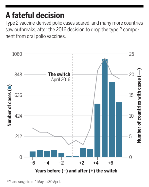 Figure 1: Reproduced from Roberts 2024.1
I became interested in the topic of vaccine virulence due to treatments after reading articles on “the switch” of oral poliovirus vaccines in April 2016, when 155 countries began use of an altered version of the classic Sabin oral poliovirus vaccine (OPV) that did not protect against Type 2 poliovirus in routine immunizations.1–3 Due to OPV being a live-virus vaccine, it can replicate and shed in stool of vaccinated individuals. It also has the rare possibility of circulating vaccine-derived poliovirus (cVDPV) after reversion to widltype pathogenicity. It has led to the reduction of over 99.9% of polio cases since 1988. After the Global Polio Eradication Initiative (GPEI) had declared the wildtype Type 2 poliovirus to be eradicated in 2015 (the last wildtype Type 2 poliovirus was observed in 1999), “the switch” was coordinated to prevent cVDPV2 as well, since it is introduced by OPV. Besides discontinuation of classic OPV, officials stockpiled an oral vaccine targeted solely to Type 2 to be used during supplementary immunization activities (SIAs) to prevent current outbreaks of cVDPV2 (OPV2), as well as started to use the killed, injected poliovirus vaccine (IPV) in Lower-and-Middle Income Countries (LMIC), which prevents disease but does not prevent transmission.
Unfortunately, children not vaccinated against Type 2 became susceptible, and cVDPV2 began to circulate among them; 3 to 4 years after “the switch,” “cases jumped from 84 in seven countries to 548 in 21 countries,” and “the number of cases has increased tenfold since 2015.”1 The catch-22 is that one needs to vaccinate as many children as possible against Type 2 in order to prevent outbreaks, yet vaccination also leads to the possibility of further cVDPV2.2 At the end of a technical report by the GPEI, an epilogue was also written: that there is a “moral imperative” to rehabilitate and educate those children who have been paralyzed, as well as to protect health-workers on the ground administering the vaccine, primarily in Pakistan, given that over 100 of them have been assassinated.1
Many vaccines are live-virus vaccines, which can provoke stronger immune responses in comparison to inactivated, or killed, vaccines. These include varicella vaccines,4 as well as, more recently, transmissible vaccines for animal populations, where the vaccine replicates within hosts is transmitted between hosts in order to provoke an immune response in hard-to-vaccinate populations. Knowing the risks of virulence evolution of these vaccines can be challenging.5
Imperfect vaccines
Virulence evolution of wildtype strains has also been extensively studied.6 When a tradeoff between infection duration and transmission is assumed as virulence increases, the optimal virulence strategy will evolve to be intermediate (rather than one of the two extremes of very high virulence or very low virulence). Ecological factors that could select for higher virulent strategies by modifying this tradeoff include imperfect vaccines, where within communities of vaccinated individuals the costs of higher virulence have been lowered since disease is prevented, but the virus can still circulate among the community, selecting for higher virulence.7 This evolutionary phenomenon has been suggested to have occurred in Marek’s disease virus.8,9 Note that this is different from a live-virus vaccine reverting to pathogenicity: the vaccine creates conditions that select for higher virulence of the wildtype strain.
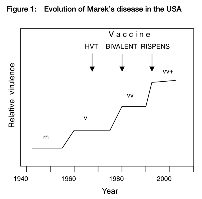 Figure 2: Reproduced from Fehler et al. 2001.9
While such theoretical models are important to identify ecological factors that may select for higher virulence, such as imperfect vaccines, they normally lack a genetic basis.10 Doubts have been raised on the generalizability of such a theoretical model,10–12 since many other factors besides virulence affect virus transmissibility and infection duration. More recent research has also proposed that case detection may be the important tradeoff factor, rather than death.13 MDV may actually represent an edge case rather than the norm given that many human infections do not exhibit this behavior.11 These reasons include:
- High crowding of birds in industrial settings.
- Vaccination is near 100%.
- Because MDV is an alpha herpesvirus, it has many anti-immune responses, allowing for multiple pathways of pathogen evolution.
Furthermore, a reason that this evolutionary phenomenon may not occur for other pathogens may come down to immunological complexity: innate immunity normally attacks conserved regions of pathogens and thus the immune response may not be evaded by evolution so easily, in comparison to the later stage of interactions with adaptive immunity.11 Opposite results, such as higher virulence giving a competitive edge to the malaria parasite within hosts, also suggest some fragility to the model: unaccounted ecological factors can flip model results. Basing policy on such a model, such as whether to use an imperfect vaccine, is then fraught with uncertainty, and may be detrimental if the evolutionary result only occurs in very specific situations, lacking generality. Although differences in virulence certainly do exist,14 assumptions of the evolutionary tradeoff, transmission model, process of evolution, and sometimes a lack of within-host modeling, can be too strong. Among these assumptions:
- Most evolutionary models assume the resident population comes to fixation before introduction of a mutant, not addressing transient dynamics. They also assume that mutations can only change virulence by a small amount in each time step, which may not be the case.
- Models that solely consider between-host transmission may be misspecified since they lack within-host processes, such as co-infection, which can flip results of the predicted impact of ecological factors such as higher host mortality.15
- The observed tradeoff between virulence and transmission, oft-assumed, is unknown for many pathogens.16
Yet the elegance of simple models, although they normally ignore within-host complexities, are rationale of their use: they are normally analyzable, giving us insight into the transmission and evolution of pathogens.17 Empirical experiments can then be done to check the predictions of the model.8 Some literature argues however that these simple evolutionary predictions must be based on other data sources, such as genetic viral sequences, even before empirical experiments.10
Call for more complex modeling approaches
Clearly, whether or not vaccines revert to virulence or select for higher virulence, and then fixate in a population, is of utmost concern. The conundrum is that these same vaccines prevent infection and mitigate widespread circulation. Part of carefully assessing the pros and cons of proposed use of a vaccine then relies on estimation of the risk of virulence evolution due to, or of, the vaccine.
Solutions to address eco-evolutionary complexities
There have been many recent developments to address the eco-evolutionary complexities of virulence evolution. There are many definitions for pathogen virulence, and implicitly this definition is host-dependent. Here, I define virulence as the host mortality rate due to disease, which may due to such within-host factors as higher replication.
Transmission modeling
An important nuance of virulence evolution is that just because virulence evolution occurs, this does not mean it will fixate in the population. In other words, it is a necessary, but not sufficient conditions for cVDPV2 emergence. A striking feature of Type 2 OPV is that it will revert to wildtype pathogenicity very quickly: on average 10 to 100 days into shedding,18 meaning that even in a single vaccination it can revert. And yet these wildtype-like strains do not always fixate in the population. We would like to know the risk factors for cVDPV2 circulation, since for example, since between “the switch” and November 2019, 300 million doses of OPV2 have been administered in response to 325 paralytic cases, leading to increases of 1800 cases of cVDPV2 in 30 countries between January 2020 and April 2022.3
Polio is an excellent system to explore these eco-evolutionary complexities because of how much we know about virulence evolution in this system:
- We know the gateway mutations of virulence.
- We know that virulence has convergent evolution, consistent with a selective advantage of high virulence.
- We already have some idea of a risk of virulence evolution (roughly 1 in 100 million exposures leads to cVDPV2 emergence)
- We have both transmission data as well as genomic data to base predictions.
- We have some idea of the tradeoff between virulence and transmission (although exceptions to the rule are possible, see Figure 3).
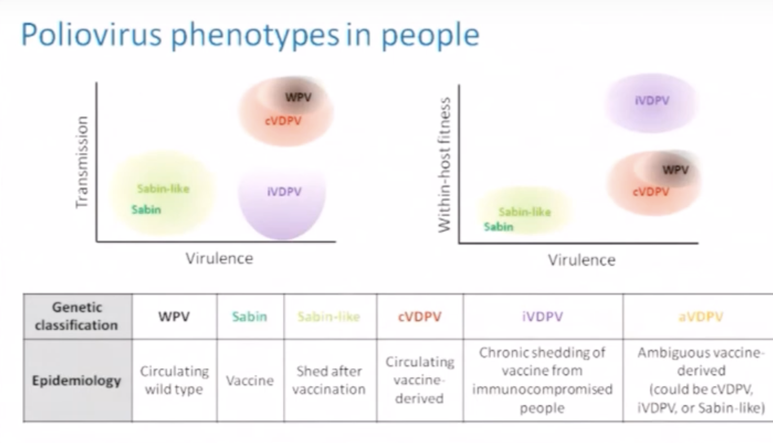 Figure 3: Reproduced from Farmulare 201818
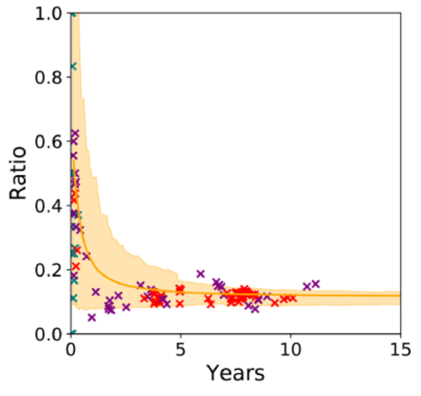 Figure 4: Reproduced from Wong et al 2023.3
There has been some research in polio to simulate both the between-host contact structure (in different communities) as well as within-host complexities of shedding duration, immunity, viral titer levels, and susceptibility.3 A transmission modeling approach, with a within-host component, may be most fruitful to understanding the conditions where virulent strains are expected to fixate. Sanitation and low-population densities for example, are key to avoiding the risk of cVDPV2. Incorporation of the dN/dS evolutionary rate (see Figure 4 below) are also key. With polio trial data, the authors went through the trouble of inferring rates of nonsynonymous and synonymous mutations, as well as of the nonsynonymous mutations, whether they were neutral or deleterious. A genotype-to-phenotype map was also created: this is most important for the gatekeeper mutations, but also deleterious mutations were calibrated to lead to a slight decrease in infectiousness (as measured and simulated with viral titer levels). Additionally, mutations that fixate earlier after vaccination have higher fitness effects than later. Probabilities of infection, via viral titer levels, increase with each gatekeeper mutation. Transmission is a function of viral shedding rate of the infecter and susceptibility of the infectee. One can see that successful circulation then depends on various epidemiological factors: if a person has the reverted strain, but does not shed at a high rate, or has a short shedding duration, or does not have necessary contacts to prolong circulation, cVDPV2 will not circulate. On the between host scale, 10% to 90% of children under 5 are vaccinated in a population of 80,000 individuals across 45 villages over approximately 3 years.
When simulating the epidemic, 40% of simulations showed stochastic die-out of epidemics. Across simulations, possible phenotypes of shedding durations and viral infectiousness varied widely due to genetic drift, and were inversely proportional to infection counts. Higher fecal-oral transmission, which can occur in unsanitary conditions, led to greater risk of cVDPV2, as did lower vaccination and boosting. Importantly, low-coverage campaigns, especially one year post-cessation of vaccination, exhibited large probabilities of outbreaks. The risk of outbreaks falls after the first year after cessation of a vaccination campaign, but steadily rises due to declining vaccination coverage. Even with so much modeling, some things are left out such as possible recombination with human enterovirus C as well as differing intra-host rates of selection.19 But the broad strokes conclusions show that the host ecology and epidemiology is fundamental to whether virulent strains are allowed to fixate in the population.
Phylogenomic approach
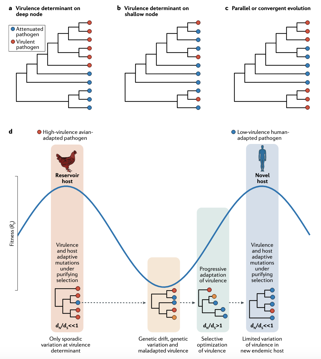 Figure 5: Reproduced from Geoghegan and Holmes 2018.10
Phylogenomic approaches can be used to identify virulence determinants, as well as the nature of virulence evolution, e..g., whether it is associated with higher fitness. The former can be done by simply matching “key branches” of an inferred phylogeny to events such as marked increase in mortality and morbidity and invasions into new geographic areas. Figure 5 shows an example of how the latter can be done.10 Specifically, if mutations are (1) associated with higher virulence fall deeper on a tree, (2) occurring multiple times in the tree (convergent evolution, (3) dN/dS is much greater than 1 during the emergence of the virulence determinant (adaptive evolution), then becomes much smaller than 1 (purifying selection). For example, if all three occur, or some combination of the three occur, this would be consistent with virulence being advantageous for the pathogen in a certain population.
Since these mutations may also be part of other evolutionary tradeoff traits if there is a positive correlation between virulence and these other traits, this would further illuminate how virulence evolution may be dependent on the tradeoffs of these other traits as well. Challenges of these types of approaches include epistatic effects, as well as that if virulence determinants are caught early, they will necessarily be closer to the tips of the phylogeny rather than the roots even if they may have a true selective advantage.
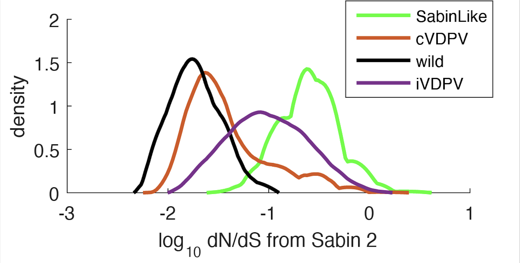 Figure 6: Reproduced from Wong et al 2023.3
In Figure 6, what this is showing are the dN/dS rates in the capsid for several strains, measured as the number of nonsynonymous changes to synonymous changes in reference to the vaccine strain. The lowest dN/dS is of the wildtype, and on the other extreme, are the Sabin-like strains, which are exploring the highest amount of amino-acid space.
References
- Leslie Roberts. Report offers harsh verdict on global polio vaccine switch. Science, 384(6696):608–609, 2024.
- Apoorva Mandavilli. The pivotal decision that led to a resurgence of polio. New York Times.
- Wesley Wong, Jillian Gauld, and Michael Famulare. From vaccine to pathogen: Modeling sabin 2 vaccine virus reversion and evolutionary epidemiology in matlab, bangladesh. Virus Evolution, 9(2):vead044, 2023.
- Judith Breuer. Molecular genetic insights into varicella zoster virus (vzv), the voka vaccine strain, and the pathogenesis of latency and reactivation. The Journal of Infectious Diseases, 218(suppl_2):S75–S80, 2018.
- Daniel G Streicker, Megan E Griffiths, Rustom Antia, Laura Bergner, Peter Bowman, Maria Vitoria dos Santos de Moraes, Kevin Esvelt, Mike Famulare, Amy Gilbert, Biao He, et al. Developing transmissible vaccines for animal infections. Science, 384(6693):275–277, 2024.
- Samuel Alizon, Amy Hurford, Nicole Mideo, and Minus Van Baalen. Virulence evolution and the trade-off hypothesis: history, current state of affairs and the future. Journal of evolutionary biology, 22(2):245–259, 2009.
- Sylvain Gandon, Margaret J Mackinnon, Sean Nee, and Andrew F Read. Imperfect vaccines and the evolution of pathogen virulence. Nature, 414(6865):751–756, 2001.
- Andrew F Read, Susan J Baigent, Claire Powers, Lydia B Kgosana, Luke Blackwell, Lorraine P Smith, David A Kennedy, Stephen W Walkden-Brown, and Venugopal K Nair. Imperfect vaccination can enhance the transmission of highly virulent pathogens. PLoS biology, 13(7):e1002198, 2015.
- Frank Fehler. Marek’s disease: History, actual and future perspectives. Lohman Inf., 25:1–5, 2001.
- Jemma L Geoghegan and Edward C Holmes. The phylogenomics of evolving virus virulence. Nature Reviews Genetics, 19(12):756–769, 2018.
- James J Bull and Rustom Antia. Which ‘imperfect vaccines’ encourage the evolution of higher virulence? Evolution, Medicine, and Public Health, 10(1):202–213, 2022.
- Dieter Ebert and James J Bull. Challenging the trade-off model for the evolution of virulence: is virulence management feasible? Trends in microbiology, 11(1):15–20, 2003.
- David A Kennedy. Death is overrated: the potential role of detection in driving virulence evolution. Proceedings of the Royal Society B, 290(1995):20230117, 2023.
- Dong-Hun Lee, Miria Ferreira Criado, and David E Swayne. Pathobiological origins and evolutionary history of highly pathogenic avian influenza viruses. Cold Spring Harbor perspectives in medicine, 11(2):a038679, 2021.
- Dieter Ebert and Katrina L Mangin. The influence of host demography on the evolution of virulence of a microsporidian gut parasite. Evolution, 51(6):1828–1837, 1997.
- Ian F Miller and C Jessica Metcalf. Vaccine-driven virulence evolution: consequences of unbalanced reductions in mortality and transmission and implications for pertussis vaccines. Journal of The Royal Society Interface, 16(161):20190642, 2019.
- Mike Boots. The need for evolutionarily rational disease interventions: vaccination can select for higher virulence. PLoS Biology, 13(8):e1002236, 2015.
- M. Farmulare. Evolutionary epidemiology of vaccine-derived poliovirus transmission. https://www.youtube.com/watch?v=83X-HwkMp3g.
- Glynis Dunn, Dimitra Klapsa, Thomas Wilton, Lindsay Stone, Philip D Minor, and Javier Martin. Twenty-eight years of poliovirus replication in an immunodeficient individual: impact on the global polio eradication initiative. PLoS pathogens, 11(8):e1005114, 2015.
-

pixelMalariaPredict
-

ThimbleTheater
-
GamesFamilyConvert
-

PushPin
-
The New Yorker
News
- Oct 2026“Challenges for the effectiveness of infectious disease interventions during global change” published in Communications Health.
- Sep 2026Semifinalist, 2026 Rising Stars in Data Science Workshop, University of Chicago.
- Feb 2026“Characterizing Newcastle disease virus transmission dynamics and the impact of vaccination in village settings” published in Proceedings of the Royal Society B: Biological Sciences.
- Aug 2025Started postdoctoral position to work on malaria hotspot prediction, Department of Global Health and Population, Harvard University.









Justin Sheen, PhD
신기현
machine learning · causal inference · public health · single-panel cartoons · running · biking · skiing · open water · nature · photography
@Harvard